A total of 24 teams came to France, with each team believing in their own philosophy, personnel, and tactics for the FIFA Women’s World Cup 2019. Although the Men’s World Cup in 2018 showed that possession-based football is not the surest possible road to a successful campaign in a knock-out competition, there are still more teams than not who believe that keeping the ball for an extended period of time is the best possible way to create chances and ultimately control matches. This philosophy requires a lot of things, foremost of which is the personality of the eleven players themselves to stay comfortable on the ball and look for.
Ball progression is essentially just that. It is the process of moving the ball through the thirds and getting the ball closer to the opponent’s goal such that it is easier for the teams to create chances. Although football is a very complex game, yet if you’re keeping the ball in the opponent’s half for a sustained period of time, it’s easier to put pressure on them while increasing your own chances of creating high-quality shots. In this data analysis piece, we’ll take a simple look at the best ball progressing midfielders from this Women’s World Cup using the Statsbomb data. As well as using data analysis we will use tactical analysis to find which players are important to their respective teams.
Objective
My objective is not to build a model in this piece. What we’ll instead do is take a simpler look at the data, play around with the passing data, and try to look at which players ultimately have the highest responsibility of progressing the play for their team.
Pre-requisites
You’ll need access to the Statsbomb data. Furthermore, I’ll be using Python and its various libraries such as Pandas, Matplotlib, and the json library (which comes built-in with Python).
Let’s get started
We’ll import the libraries first. I’m using Jupyter Lab, although you may use any IDE of your choice. Nothing is really different in that regard (except for some very minor changes).
import pandas as pd import matplotlib.pyplot as plt import json from pandas.io.json import json_normalize import matplotlib matplotlib.style.use("ggplot")
Now we’ll go ahead and try to read in the data from the Statsbomb repository. The way it works is that they’ve got all their event data in a single file – the events file. It contains data from the FIFA 2018 World Cup, the FA WNL, and the ongoing WWC 2019. This makes it impossible to iterate through the whole folder and get only the matches from WWC 2019. Hence, we’ll have to go to the matches folder – which contains the match ids of all the matches for specific competitions and then get the ‘ids’ from there. Then we use those ids to go to then get into the events folder and get only the matches we are interested in.
with open (r"C:\Users\ADMIN\Desktop\Abhishek\open-data\data\matches\72.json", "r") as f: obj = json.load(f) mlist = [] objlist = [] dflist = [] for match in obj: mid = match["match_id"] mlist.append(mid) mlist = [str(m) for m in mlist] mlist = [m+".json" for m in mlist] for n in mlist: file = "C://Users/ADMIN/Desktop/Abhishek/open-data/data/events" + "/" + n with open (file, "r") as f: obj = json.load(f) objlist.append(obj)
Now, we’ve got a list of Pandas dataframes for all the separate matches. We’ll now proceed to merge the dataframes into one master dataframe containing all the events from the World Cup till date. Here’s how we do that
for obj in objlist: df = json_normalize(obj) dflist.append(df) result = pd.concat(dflist, sort=True)
Now we have our result dataframe ready.
Note: I’ll call the “result” dataframe “df” for the rest of the post
The first thing we do now is to filter only the passes from the dataframe. Next, we’ll notice that the location for the starting and ending of the passes are in a list under the columns – “location”, “pass.end_location”. Great. We can now create four more columns from these two columns, namely – “Start X”, “Start Y”, “End X”, and “End Y”.
We’ll do that as follows
df = result[result["type.name"]=="Pass"] df[['Start X','Start Y',’End X’,’End Y’]] = pd.DataFrame(df[[“location”,”pass.end_location”]].values.tolist(), index= df.index)
To understand ball progression, we need to understand the pitch dimensions first. Since a pitch is measured in terms of x, y-axes, where x is the length and y is the width, most of our data crunching will be focused on the x-axis.
The first thing to do is to create a difference column which measures the difference between the ending and starting x coordinates of every pass. We’ll also set the negative values to zero – that is a back pass has no effect on the total score since we’re only considering passes that move the team up the pitch.
df["X-difference"] = (df["End X"] - df["Start X"]).clip(lower=0)
Next, we’ll filter the dataframe some more. We only have passes now but we’ll go ahead and drop all the set-pieces, kick-offs, throw-ins. This is so that only regular play is considered.
This is also where we’ll consider only successful passes. Here’s where I am making a big assumption – I’m working under the premise that if the pass.outcome.name was nan, it was a successful pass. The Statsbomb docs weren’t entirely clear on this area and that might be worth keeping in mind.
df.drop(df[(df["play_pattern.name"]=="From Kick Off")|(df["play_pattern.name"]=="From Free Kick")|(df["play_pattern.name"]=="From Throw In")|(df["play_pattern.name"]=="From Corner")].index, inplace=True) df = df[df["pass.outcome.name"].isna()]
Now, we’ll aggregate the sum of all the difference in x we calculated earlier for every player. We’ll use Pandas’s life-saver function groupby for that. Then we set a filter for the minimum duration played by the player. This is akin to setting a lower filter for the number of minutes played by a player, to weed out inflated stats, if any. We’ll also need the sum of duration later, which we’ll get to in just a second.
gdf = df.groupby(["player.name"])[["X-difference", "duration"]].agg("sum") gdf = gdf[gdf["duration"]>120] gdf["Progression per 90"] = (gdf["X-difference"]/gdf["duration"])*90
We then multiply that value with 60 because the duration value is in seconds and it might be easier to understand if the data we get is in minutes. So essentially, we’re talking about how much pitch an individual player gains via a pass per minute of possession.
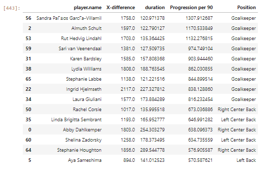
As expected, the top players are almost exclusively goalkeepers. This is because they usually are expected to clear their lines and those contribute a lot to getting higher ball progression values. So we can go ahead and remove all the goalkeepers from our df to gain better insight into the lesser-known players of the team. In fact, we should remove all the defenders as well because they aren’t necessarily known for progressing the ball. More importantly, their progression score will be affected by the clearances and long balls – particularly because, Statsbomb don’t tag clearances in the pass data. Keep in mind that our initial objective was to find midfielders who are good at progressing play and so we can safely go ahead and remove them all.
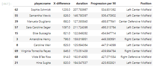
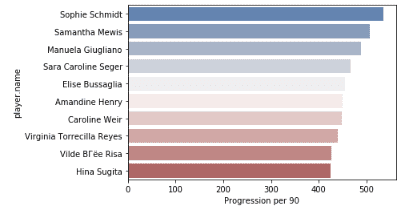
Now we’re finally getting somewhere. We’ve got quite a few interesting new names – as well as certain expected ones in terms of Amandine Henry and Sophie Schmidt. If we visualise that in a bar plot, here’s what we get.
Now, let’s look at the passes for any random player from this list.
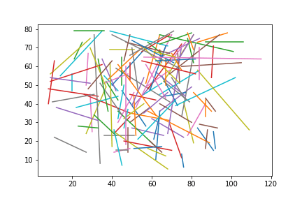
We can see quite a few long balls. Especially, from the right side of the pitch. We also see a few cross-field diagonals but those weren’t reflected in our model since we weren’t considering changes in y; only in x.
Now let’s go ahead and find out the most prolific players from every team. We’ll again use groupby and group on the country as well as the player. Then we’ll choose the top player from every team.
All of this can be done in a one-liner which goes like this:
teamdf = df.groupby(['team.name', 'player.name'])[["X-difference", "duration"]].agg("sum").reset_index()
This is our end result.
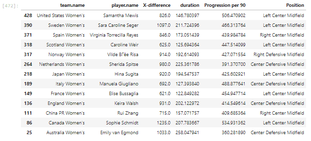
Finally, a bar plot of these players to wrap everything up.
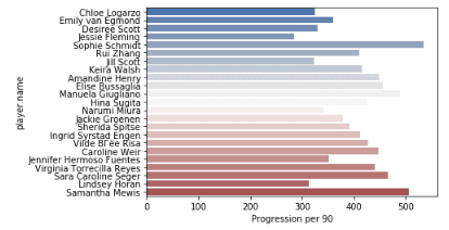
Conclusion
There are quite a few caveats that are associated with creating a progression model using x,y event data. They lack a lot of context and a lot of events might be missed or not wrongly tagged. However, this is not bad for a first attempt. In later stages, we can focus on filtering out clearances and ensuring that we can inaccurate passes and accurate passes are correctly tagged and dealt with. I also hope this piece acted as a primer on how easy it is to crunch large sizes of data in an efficient manner in Python and how easy it is to build models.
If you love tactical analysis, then you’ll love the digital magazines from totalfootballanalysis.com – a guaranteed 100+ pages of pure tactical analysis covering topics from the Premier League, Serie A, La Liga, Bundesliga and many, many more. Buy your copy of the June issue for just ₤4.99 here, or even better sign up for a ₤50 annual membership (12 monthly issues plus the annual review) right here.




Comments